Cover image owned by: https://www.activestate.com/
One way to continue learning in the world of Data Science is to stop by Kaggle and try to participate in one of the competitions held there.
That is the case that we address here, but I want to focus especially on the use of Pipelines for model automation. This is a powerful aspect within the methods available in Sklearn and that once the model is trained, allows you to various options more efficiently and with fewer lines of code such as linking various common stages of data preprocessing, optimizing hyperparameters, analyzing overfits by cross-validation, decreasing dimensionality so that the model generalizes better, which also helps to improve processing performance by needing fewer memory resources, etc. All this brings development closer to production, being able to automate all stages of the training process and successive tests in a more efficient way.
Taking advantage of the development carried out for the competition that I mentioned earlier in Kaggle, I stumbled upon the need to decrease the dimensionality of the data set, as it was hugely heavy with more than 2.5 million records and 130 variables and the rules impose a limited execution time for the processing of the model. This caused you to use Principal Component Analysis (PCA) to decrease variables in components and decrease memory needs. Taking advantage of this learning, I have tried to collect this process by using it in this post to be able to have at hand, a case of use of the Pipeline method, cross-validation and dimensionality reduction, which are usually used together in many cases by their automation power.
Here we will therefore explain a use case, but if you want to expand on the information you can consult the complete notebook that I have developed with different options that are most commonly used in this process and that serves me as a kind of cheat sheet to consult in the development of these cases.
When you finish reading this post, you will have an idea of using pipelines, transformers for preprocessing, reducing dimensionality with Principal Component Analysis (PCA), using cross-validation to counter overfit and hyperparameter optimization.
We started by describing the data and what Jane Street Market Prediction’s challenge was in Kaggle. The provided dataset contains a set of 130 variables, representing actual stock market data. This is a fairly heavy Dataset (5GB) with more than 2 million records, where each row in the dataset represents a trading opportunity, for which we will be predicting: 1 to make the buy trade and 0 not to do it. Each operation has an associated weight variable and 5 «resp» variables from 0 to 4, representing returns on different time horizons. In the test suite to evaluate model performance, we didn’t have «resp» values so we have to use only the 130 features (feature_n) to make the prediction.
To be more efficient when exposing this post, we’ll extract a small portion of the data to see how the defined model behaves.

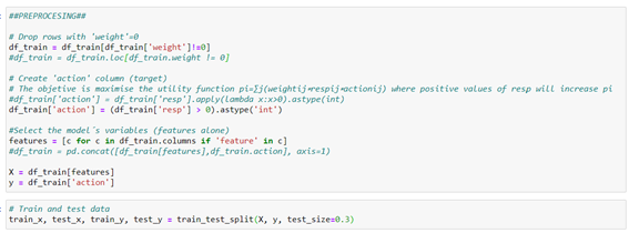
We pre-process the data according to the requirements of the competition. We discard the records with a weight of 0, we define the target variable as 1 when the resp variable is positive and 0 the rest of the cases. We select only the variables “feature_n” that is with which the prediction will be made. We will divide into train and test to do the overfit checks of the model.
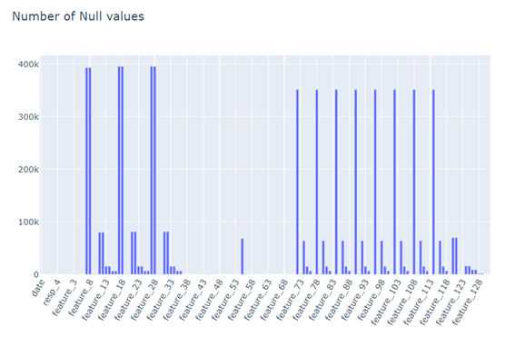
It´s verified that there are many records with missing values:
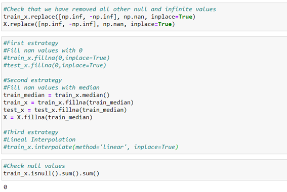
Therefore, we´ve to manage null values. As an approximation, we use the strategy of replacing null values with the median of all values in the variable. Perhaps we would get a somewhat better result with linear interpolation when the data came from a time series and the missing value would be more influenced by the nearby values. But to simplify and focus on the purpose of the post, we use the median to have a first approximation.
We start from a basic ExtraTreeClassifier model, chosen after a comparative pre-analysis of the performance of different models. You can view the notebook where this comparison is made from the project website on Github.
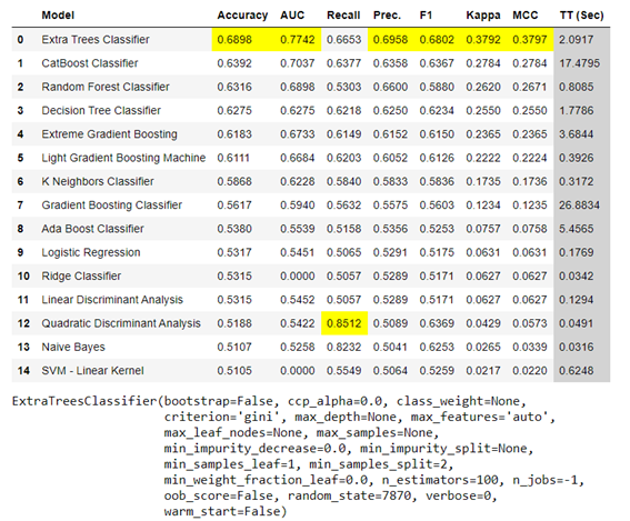
Previously we generated a function to automate the performance metrics of the models that we are going to test.
We coded the basic model.
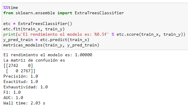
We tested on the test dataframe.
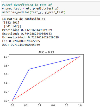
Excessive overfit can be seen in the generated model (AUC = 1 vs. 0.73).
To try to improve the testing process, let’s:
- Automate the process with Pipeline and Transformers.
- Feature selection and dimensionality reduction (now 130 variables). To generalize the model and decrease the processing time.
- Cross-validation to select hyperparameters and decrease overfit.
- Channel all these processes in a single operation.
Process Automation | Pipeline
Sklearn has methods to pipe in a single step all the threads that can be developed in a modeling and that help to bring it to production or improve it: From the preprocessing of the data (which we have done previously), the application of these based on the type of columns (transformers), standardization, selection of characteristics, reduction of dimensionality to finally the model to be trained (estimator).
- Transformers
- Imputation of missing values
It´s possible to preprocessing the data with these standard transformers that come by default in Sklearn (called estimators) or also make them more personalized. This will allow preprocessing to be part of and integrate into the entire model to be trained.
The transformation method must begin by choosing the characteristics/columns relevant to the transformation (for example, numeric characteristics, categorical characteristics, or columns with a common name). Most commonly they are grouped by numerical columns on one side and categorical on the other.

In our use case, we will make a one-way allocation of the median to the missing values in all columns, using the estimator SimpleImputer that only replace the lost value with another fixed value, in this case, the median: SimpleImputer(missing_values=np.nan, strategy=’mean’ o ‘median’)
- Normalize data
In many cases, it´s necessary to normalize the data or standardize it on a common scale as a pre-process to all other operations. In our case how we are going to do a reduction in the dimensionality this previous step in the numeric characteristics is necessary. We use StandardScaler() that eliminates the mean and applies the unit variance.

Now we need to tell you which columns or variables these transformations will be applied to, for which we use the instance ColumnTransformer() formatted:
ColumnTransformer(transformers=[(‘ chosen name’, trasformer, [‘ columns list to be applied ‘])]
In our case we apply:

It joins all preprocessing with the chosen prediction model into a single pipeline and we measure performance:
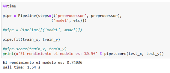
For now we get a slightly smaller overfit than applying the model directly. We’re going to keep improving the process.
- Reduced unsupervised dimensionality
We have used Principal Component Analysis (PCA) with the composition.PCA() method is available in Sklearn, which tries to look for a combination of features (components) that capture well the variation of the original features. This is the most widely used method to reduce dimensionality. In this case, we managed to reduce from 130 variables to 14 components that explain 90% of the variance of the target variable.

With these 14 components that explain a good percentage of predictive power, we introduce it into the pipeline we are developing:
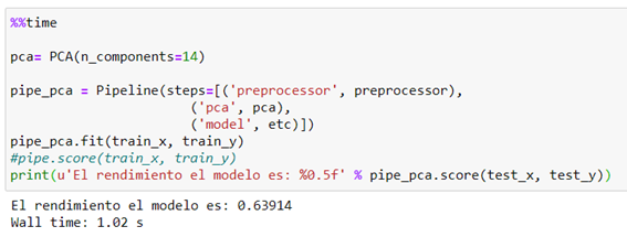
We have reduced to 14 components obtaining slightly lower performance of the model, but having reduced the processing speed by almost 34%. This means that by scaling it to all data we will get a more time-free processing time.
At this point, an overfitting model between training and validation data is observed, so cross-validation is convenient to reaffirm the results and see what performance is like in this case.
First, we do a model performance check-in cross-validation, before introducing it into the pipeline. To do this we use the cross_val_score operator, which will tell us in a quick and more approximate way how the model will behave with external data. We´ll use the default strategy which is K-fold by default when we put an integer in the «cv» argument.
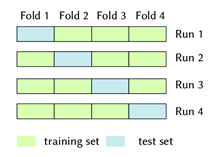

How we can see slightly decreases the accuracy to 0.6 with a typical deviation of 0.05.
Let’s try to improve that performance using a more demanding iterator, although this can be computationally more expensive. In this case, we use the RepeatedStratifiedKFold iterator that repeats the tiered K-Fold ‘n’ times with different randomization in each repetition.

This iterator checks for a substantial performance improvement, although it is a computational time cost of 32%.
Join of the different parts
Once the Pipeline is defined, we move on to improving the model using the GridSearchCV or RandomizedSearchCV objects to obtain the most appropriate hyperparameters, so, to optimize the model.
In this case, we optimize three parameters and use ShuffleSplit cross-validation iterator, which will generate a user-defined number of test dataset divisions in this case we have defined 75% for 5 iterations. Samples are mixed again randomly in the next iteration and so on. With this process, we hope to reduce overfit and improve the generalization of the model.
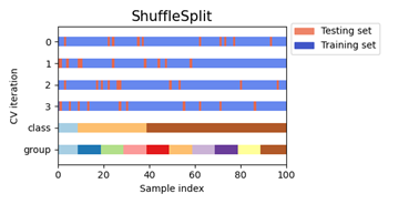
We check the performance and the overfit of the final model:
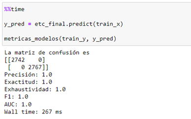
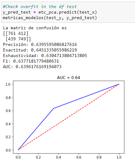
You can see a decrease in the performance of the original model (AUC 0.73 vs. 0.64) but greater generalization with external data and a shorter execution time of the process when scaling into massive data that is decisive in this Kaggle competition in which processing times are restricted in order to finish the challenge.
If you want to see the complete process of participation in the competition, you can consult the notebook at de Kaggle.
For the collection of tips for using Pipeline, cross-validation, feature selection, decreased dimensionality and optimization of Models, you can consult my own ‘cheat sheet’ on the project website on Github.

