
In this analysis, I will use a set obtained in a study of a population of children that in which their habits have been followed looking for the characteristics that can predict the appearance of myopia. The different predictive classification models will be studied for the best performance.
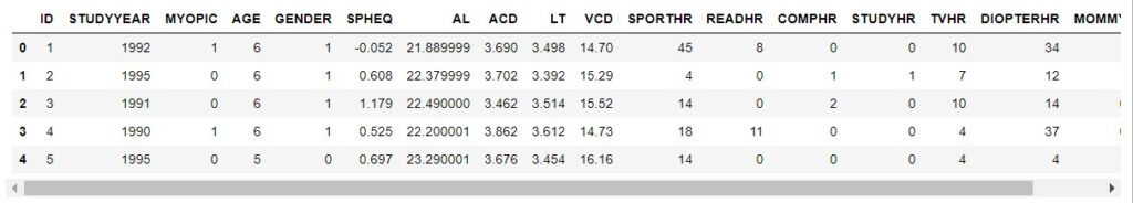
The dataset is a subset of data from the Orinda Longitudinal Study of Myopia (OLSM), a cohort study of ocular component development and risk factors for the onset of myopia in children. Data collection began in the 1989–1990 school year and continued annually through the 2000–2001 school year. All data about the parts that make up the eye (the ocular components) were collected during an examination during the school day. Data on family history and visual activities were collected yearly in a survey completed by a parent or guardian. The dataset used in this text is from 618 of the subjects who had at least five years of follow-up and were not myopic when they entered the study. All data are from their initial exam and the dataset includes 17 variables. In addition to the ocular data, there is information on age at entry, year of entry, family history of myopia and hours of various visual activities. The ocular data come from a subject’s right eye.
The dataset “myopia.csv” is collected from https://rdrr.io/github/emilelatour/purposeful/man/myopia.html:
A data frame with 618 observations and 18 variables (see the meaning of each variable in my web poject in Github). With this data, you can create a model that can predict the occurrence of myopia in the study set. The first step for them is to import the data.
We pre-explore the data using a histogram of each variable:
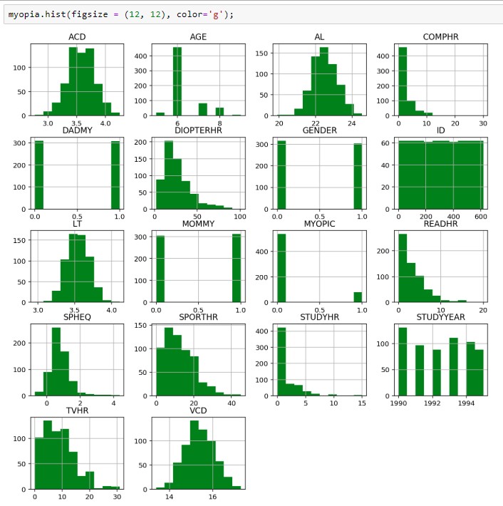
There are multiple binary characteristics (DADMY, GENDER, MOMMY, MYOPIC), one identified (ID), two categorical variables (AGE and STUDYYEAR) and the rest are continuous variables.
On the other hand, you can use the scatter_matrix function to check the relationships of correlations between the different characteristics.
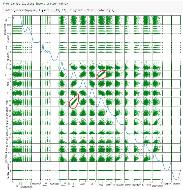
There are several features where there is a clear correlation, for example, VCD-AL.
Feature selection
Starting you can get a list with independent characteristics and another list with the target feature to apply in machine learning algorithms.
We can note four categorical features (AGE, GENDER, MOMMY, DADMY) and all of them are binary, except AGE feature that has several levels and I need to create a type dummy in this feature.
Elimination of collinear features
As we can see in the initial scan, we can see collinearity between some variables so we try to eliminate those variables to reduce the dimensionality of the data frame. We can use VIF (Variance inflation factor) method, measure how much the variance of the estimated regression coefficients are inflated as compared to when the predictor variables are not linearly related.
It is important here to note that All the features should be numeric.
As a thumb rule, any variable with VIF > 2 is avoided in a regression analysis. Sometimes the condition is relaxed to 5, instead of 2.
We create a function that allows us to automate the process of deleting variables with a VIF > 5.
It can be seen that there is large multicollinearity between the different characteristics of the model. In fact, there are several features with Infinite VIF, indicating perfect multicollinearity. You can use the algorithm to select only those that have a VIF less than 5.
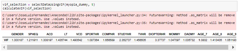
It is noted that only 15 characteristics of the 18 initials remain.
In order to better generalize the predictive model, we will continue to reduce the dimensionality of the data frame through the Selection of the best candidates. SelectKBest is a scikit-learn method can be used to select the best candidates. In this case, when working with a classification problem, the indicated f_classif must be used. In the next step, you can select the 8 best.
Creating predictive models
Previously we will create a function to automate the measurement of the performance metrics of each model.
Before starting model creation, it is necessary to separate the sample into one for training and one for validation dataset with train_test_split method of Scikit-learn.
We’re going to use traditional models to check the performance we get:
- Logistic regression
- Decision trees
- Random Forest
- SVM (Support Vector Machines)
- Knn (k-Nearest Neighbor)
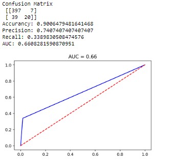
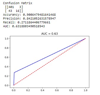
1. Logistic Regression
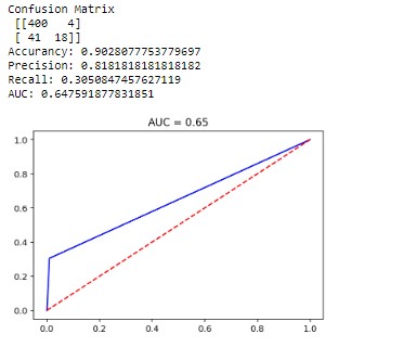
2. Decision trees
The optimal depth is around 8 but there is high overfitting. To decrease the overfitting we would have to go to a depth of 2 but we show performance results similar to the line regression.
NOTE: In another post, I will write about a visual method to define the best depth for the models.
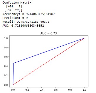
3. Random Forest
For less overfitting and better performance, we need to set a depth around 4, but the model doesn’t find better performance than the previous ones.
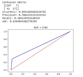
4. SVM (Support Vector Machines)
5. Knn (k-Nearest Neighbor)
Initially, you can use a value of 3 neighbours and we test to see which results it gives us the best result and less overfitting.
Finally, we run the same codes for each model with the validation dataset to check the overfitting of the model.
Summary (train/validation dataset):
- Logistic Regression = .66/.63
- Decision tres = .65/.61
- Random Forest = .73/.63
- SVM = .64/.60
- Knn = .63/.59
The best performance we get with Random Forrest but with some overfitting. It seems that the most balanced is the traditional logistic regression.