Selecting predictive features in binary classification models – Weight of Evidence (WOE) and Information Value (IV)
In this post, we’ll try to address a methodology for selecting the best predictive features for a binary classification model based on Weight of Evidence (WOE) and Information Value (IV) concepts and how they are used in the predictive modelling process along with details of how to implement code in Python on an example of urinary system disease diagnosis.
Achieving robust and well-generalized models depends on simplifying or selecting the characteristics or variables to consider for training the model and for this purpose, the weight of evidence (WOE) and the value of the information (IV) are one of the statistical techniques based on a logistic regression model most commonly used to solve binary classification problems.
These two complementary models evolved from the same logistic regression technique, developing decades ago to address different problems such as credit rating with the aim of predicting the likelihood of defaulting on a loan, clicking on an ad, cancelling a subscription, etc. So, we can say that WOE and IV play two distinct but complementary roles for transforming and screening the characteristics of binary classification models. WOE describes the relationship between a predictive variable and a binary target variable and IV measures the strength of that relationship.
Weight of Evidence – WOE
WOE is a simple but powerful technique for representation and evaluation of characteristics in data science. WOE can provide interpretable transformation to categorical and numerical characteristics. It will serve to group both categorical and continuous variables into different containers or groupings that have at least 5% of the data, so that it generates dummy variables that better describe the predictor relationship between the existing characteristics and the target variable.
By developing predictive models with these new variables using the appropriate and well-distributed grouping technique across containers, you often improve model performance by handling lost values and outliers, and you can avoid using other dummy variables. Care must be taken when dealing with missing values and grouping them separately.
In this particular case in which we will try to predict the diagnosis of two diseases of the urinary system, only WOE will serve as an intermediate calculation to obtain the IV.

Information Value – IV
Classically, this method serves as a variable classification model and allows us to make a selection of features, which is less computationally demanding than other methods. The IV of a predictor or characteristic in a classification model is related to the sum of absolute values for global WOE groups. Therefore, it expresses the amount of information in a predictor variable to separate in bivalent variables. Classifies variables according to their importance or the amount of information it carries. The value of the information increases as containers increase for a separate variable.

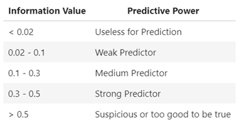
The interpretation of the results in each characteristic of the dataset can be done from this reference table:
After so much theory, let’s go to your practical application to select features. Let’s try to generate a diagnostic model of acute inflammations of the urinary bladder from a dataset supplied by the UCI that we have called «diagnostic», where we find one continuous variable and six binary variables (a1-a6) and two independent variables or targets (d1 and d2). A pre-preparation of the dataset that you can query in the project notebook on Github has been done, including the details and names of each of those variables.
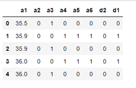
We pre-check the data:
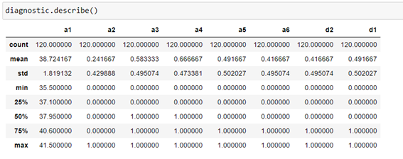
We try to check in a first approximation the shape of the data using the histogram of the different variables.
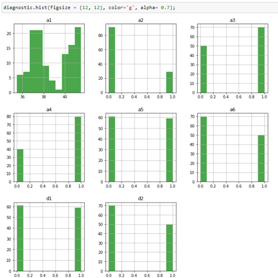
As you can see these are five binary variables and a continuous variable that corresponds to the body temperature of the patients.
We note the collinearity of the variables.
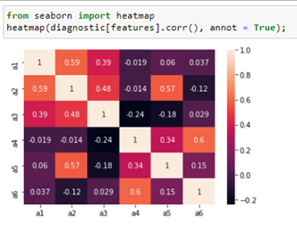
There doesn’t seem to be a correlation between the variables we can delete.
According to the formulas described at the beginning of this post, we developed two functions to calculate WoE and IV:
Referencia: Quick Guide to Pandas Pivot Table & Crosstab - Medium blog
The get_WoE function uses the panda cross-table method to group and count cases 1 or 0 (Event/No Event) and then apply the WoE formula for the Neperian logarithm of the percentage of ones (events) versus the percentage of zeros (non-events).
In the function for IV calculation (calculateIV), we incorporate the WoE calculation for each of the independent variables, applying the formula defined above in this post.
Before applying these functions to our dataset, we must meet at least two requirements mentioned at the beginning:
- The dataset must be clean. Missing data must be labelled np.nan.
- There should be no continuous attribute. Continuous attributes should be grouped into 5 to 10 containers as dummies variables, making sure that each container has at least 5% of observations.
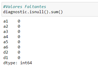
as it has been previously treated
Therefore, the first point is met in the absence of missing values.
We determine what are the independent characteristics and the objective variables, which in this case are two binary variables.

For the second requirement, we will differentiate the continuous (a1) from the categorical variables (rest).

From here, and being a case with two target variables, you’ll have to select the best predictor characteristics for each of the two independent variables.
To do this, we calculate the IV of the variables for the target_1 and on the other hand for the target_2.
We calculate IV for the first target variable (target_1):

We interpret the values obtained from IV: Below 0.1 can be a bad predictor. Therefore, we can delete the variable a6.

We calculate IV for the second target variable (target_2):

variables with respect to the second target variable
In this case none of the variables are below 0.1 so we consider them good predictors. IV values can be considered average or higher.
Treatment of the continuous variable:
We analyze the temperature variable a1 to determine whether it can be discretized or entered directly into each of the models.
We must do the analysis separately for each of the two target variables (target_1 vs target_2)
Target_1
We represent the relationship of variable a1 to target_1 using a histogram so that we can analyze whether there is any linear relationship or you can group the records into different containers based on the number of cases.
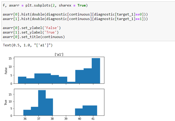
In this case you can see that the prediction depends on the variable a1 (temperature) nonlinearly, there are at least 4 categories in which the records could be grouped: up to 37ºC, from 37ºC to 38ºC, from 38ºC to 40ºC and more than 40ºC.
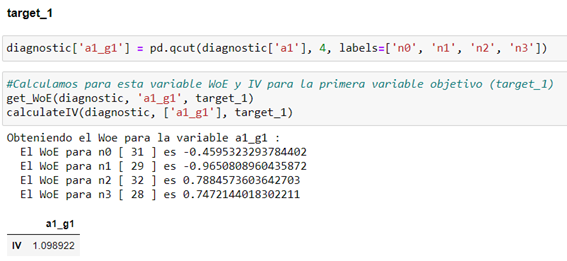
From this analysis, we generate a dummy variable with 4 classes. We do this using two methods, one of them automatic with the method. pandas’ own .qcut and the second a grouping directed by the lambda function. We check which of the two methods provides us with the best WoE and IV with respect to target_1.
- Automatic method (a1 with respect to target_1)
- Targeted method (a1 with respect to target_1)

It seems that the targeted method (variable of a1_g1_b) is more suitable, since this type of discretization provides us with a tighter IV. You can note a IV greater than 1 may be too good to be true.
Target_2
Now we do the same exercise, representing with the same type of histogram the same way the relationship of variable a1 with the target_2.
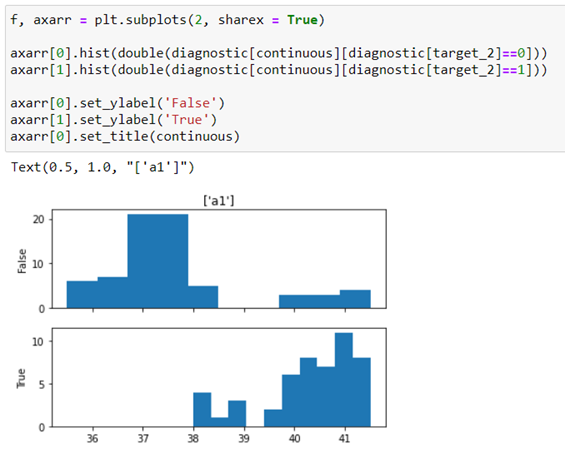
In this case we can see that you can group the records of variable a1 into two containers: less than 39 and from 39ºC.
We regroup under the two automatic and targeted methods:
- Automatic method (a1 with respect to target_2)
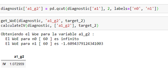
- Targeted method (a1 with respect to target_2)

In this case the automatic method seems a better predictor for discretizing variable a1.
Therefore, to generate the predictive model, we will use the variables:
- a1_g1_b for target 1
- a1_g2 for target 2
Once the continuous variable a1 has been discretized and chosen the best distribution that explains the two target variables, we generate the dummies variables in the final two datasets to create the predictive model.
Detection of multicolinearity in variables
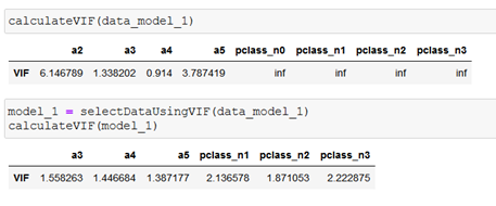
Line variables can be removed by using Variance Inflation Factor (VIF):
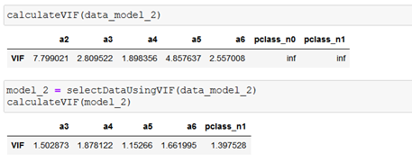
These are two functions, the first calculates the VIF of each variable, according to the definition of the Variance Inflation Factor and the second generates the dataset selecting only the variables whose VIF is less than 5 which indicates low collinearity.
- Model 1 for the first target variable (target_1)
- Model 2 for the second target variable (target_2)
Creating and validating predictive models
This is a binary classification problem so we use a logistic regression model using cross-validation. We first create the functions with the metrics needed to evaluate the models:
In this case, a typical error is to use the previously separated training datasets (x_train, x_test, y_train, y_test, etc.). Because cross-validation already separates the data into the specified number of sets and validates with data that the model has not seen, all complete data (model_1 and model_2) must be used.
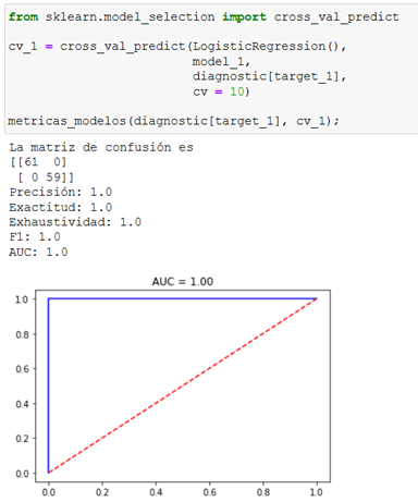
Now we analyze the performance for the modelo_2:
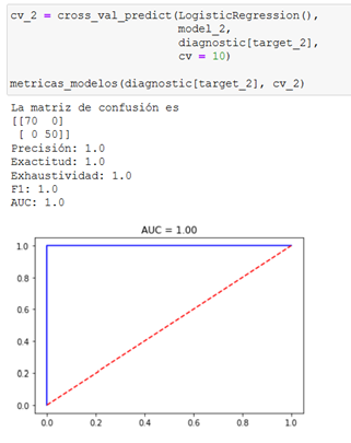
When performing models using cross-validation, you can see that the results are optimal for both target variables.
Conclusions
I know of an attribute selection method that doesn’t do enough resource computing and perhaps not too glamorous but efficient applied to binary classification models.
Using WoE method can be outliers in case of continuous variables when converting in dummies and treating them grouped into different classes. You can also edit null values by grouping them into the same class.
IV is one of the most useful techniques for selecting important variables in a predictive model. It helps variables based on their importance and is designed for the binary logistic regression model.
More details in the Github web project

